In Spring 2016 I was taking 18.757 Representations of Lie Algebras. Since I knew next to nothing about either Lie groups or algebras, I was forced to quickly learn about their basic facts and properties. These are the notes that I wrote up accordingly. Proofs of most of these facts can be found in standard textbooks, for example Kirillov.

1. Lie groups

Let $K = \mathbb R$ or $K = \mathbb C$, depending on taste.

Definition 1. A Lie group is a group $G$ which is also a $K$-manifold; the multiplication maps $G \times G \rightarrow G$ (by $(g_1, g_2) \mapsto g_1g_2$) and the inversion map $G \rightarrow G$ (by $g \mapsto g^{-1}$) are required to be smooth.

A morphism of Lie groups is a map which is both a map of manifolds and a group homomorphism.

Throughout, we will let $e \in G$ denote the identity, or $e_G$ if we need further emphasis.

Note that in particular, every group $G$ can be made into a Lie group by endowing it with the discrete topology. This is silly, so we usually require only focus on connected groups:

Proposition 2 (Reduction to connected Lie groups)

Let $G$ be a Lie group and $G^0$ the connected component of $G$ which contains $e$. Then $G^0$ is a normal subgroup, itself a Lie group, and the quotient $G/G^0$ has the discrete topology.

In fact, we can also reduce this to the study of simply connected Lie groups as follows.

Proposition 3 (Reduction to simply connected Lie groups)

If $G$ is connected, let $\pi \colon \widetilde G \rightarrow G$ be its universal cover. Then $\widetilde G$ is a Lie group, $\pi$ is a morphism of Lie groups, and $\ker \pi \cong \pi_1(G)$.

Here are some examples of Lie groups.

Example 4 (Examples of Lie groups)

• $\mathbb R$ under addition is a real one-dimensional Lie group.
• $\mathbb C$ under addition is a complex one-dimensional Lie group (and a two-dimensional real Lie group)!
• The unit circle $S^1 \subseteq \mathbb C$ is a real Lie group under multiplication.
• $\operatorname{GL}(n, K) \subset K^{\oplus n^2}$ is a Lie group of dimension $n^2$. This example becomes important for representation theory: a representation of a Lie group $G$ is a morphism of Lie groups $G \rightarrow \operatorname{GL}(n, K)$.
• $\operatorname{SL}(n, K) \subset \operatorname{GL}(n, K)$ is a Lie group of dimension $n^2-1$.

As geometric objects, Lie groups $G$ enjoy a huge amount of symmetry. For example, any neighborhood $U$ of $e$ can be “copied over” to any other point $g \in G$ by the natural map $gU$. There is another theorem worth noting, which is that:

Proposition 5. If $G$ is a connected Lie group and $U$ is a neighborhood of the identity $e \in G$, then $U$ generates $G$ as a group.

2. Haar measure

Recall the following result and its proof from representation theory:

Claim 6. For any finite group $G$, $\mathbb C[G]$ is semisimple; all finite-dimensional representations decompose into irreducibles.

Proof: Take a representation $V$ and equip it with an arbitrary inner form $\left< -,-\right>_0$. Then we can average it to obtain a new inner form $$\left< v, w \right> = \frac{1}{|G|} \sum_{g \in G} \left< gv, gw \right>_0.$$ which is $G$-invariant. Thus given a subrepresentation $W \subseteq V$ we can just take its orthogonal complement to decompose $V$. $\Box$

We would like to repeat this type of proof with Lie groups. In this case the notion $\sum_{g \in G}$ doesn’t make sense, so we want to replace it with an integral $\int_{g \in G}$ instead. In order to do this we use the following:

Theorem 7 (Haar measure)

Let $G$ be a Lie group. Then there exists a unique Radon measure $\mu$ (up to scaling) on $G$ which is left-invariant, meaning $$\mu(g \cdot S) = \mu(S)$$ for any Borel subset $S \subseteq G$ and “translate” $g \in G$. This measure is called the (left) Haar measure.

Example 8 (Examples of Haar measures)

• The Haar measure on $(\mathbb R, +)$ is the standard Lebesgue measure which assigns $1$ to the closed interval $[0,1]$. Of course for any $S$, $\mu(a+S) = \mu(S)$ for $a \in \mathbb R$.
• The Haar measure on $(\mathbb R \setminus \{0\}, \times)$ is given by

$$\mu(S) = \int_S \frac{1}{|t|} dt.$$ In particular, $\mu([a,b]) = \log(b/a)$. One sees the invariance under multiplication of these intervals.

• Let $G = \operatorname{GL}(n, \mathbb R)$. Then a Haar measure is given by $$\mu(S) = \int_S |\det(X)|^{-n} dX.$$
• For the circle group $S^1$, consider $S \subseteq S^1$. We can define

$$\mu(S) = \frac{1}{2\pi} \int_S d\varphi$$ across complex arguments $\varphi$. The normalization factor of $2\pi$ ensures $\mu(S^1) = 1$.

Note that we have:

Corollary 9. If the Lie group $G$ is compact, there is a unique Haar measure with $\mu(G) = 1$.

This follows by just noting that if $\mu$ is Radon measure on $X$, then $\mu(X) < \infty$. This now lets us deduce that

Corollary 10 (Compact Lie groups are semisimple)

$\mathbb C[G]$ is semisimple for any compact Lie group $G$.

Indeed, we can now consider $$\left< v,w\right> = \int_G \left< g \cdot v, g \cdot w\right>_0 dg$$ as we described at the beginning.

3. The tangent space at the identity

In light of the previous comment about neighborhoods of $e$ generating $G$, we see that to get some information about the entire Lie group it actually suffices to just get “local” information of $G$ at the point $e$ (this is one formalization of the fact that Lie groups are super symmetric).

To do this one idea is to look at the tangent space. Let $G$ be an $n$-dimensional Lie group (over $K$) and consider $\mathfrak g = T_eG$ the tangent space to $G$ at the identity $e \in G$. Naturally, this is a $K$-vector space of dimension $n$. We call it the Lie algebra associated to $G$.

Example 11 (Lie algebras corresponding to Lie groups)

• $(\mathbb R, +)$ has a real Lie algebra isomorphic to $\mathbb R$.
• $(\mathbb C, +)$ has a complex Lie algebra isomorphic to $\mathbb C$.
• The unit circle $S^1 \subseteq \mathbb C$ has a real Lie algebra isomorphic to $\mathbb R$, which we think of as the “tangent line” at the point $1 \in S^1$.

Example 12 ($\mathfrak{gl}(n, K)$)

Let’s consider $\operatorname{GL}(n, K) \subset K^{\oplus n^2}$, an open subset of $K^{\oplus n^2}$. Its tangent space should just be an $n^2$-dimensional $K$-vector space. By identifying the components in the obvious way, we can think of this Lie algebra as just the set of all $n \times n$ matrices.

This Lie algebra goes by the notation $\mathfrak{gl}(n, K)$.

Example 13 ($\mathfrak{sl}(n, K)$)

Recall $\operatorname{SL}(n, K) \subset \operatorname{GL}(n, K)$ is a Lie group of dimension $n^2-1$, hence its Lie algebra should have dimension $n^2-1$. To see what it is, let’s look at the special case $n=2$ first: then $$\operatorname{SL}(2, K) = \left\{ \begin{pmatrix} a & b \\ c & d \end{pmatrix} \mid ad - bc = 1 \right\}.$$ Viewing this as a polynomial surface $f(a,b,c,d) = ad-bc$ in $K^{\oplus 4}$, we compute $$\nabla f = \left< d, -c, -b, a \right>$$ and in particular the tangent space to the identity matrix $\begin{pmatrix} 1 & 0 \\ 0 & 1 \end{pmatrix}$ is given by the orthogonal complement of the gradient $$\nabla f (1,0,0,1) = \left< 1, 0, 0, 1 \right>.$$ Hence the tangent plane can be identified with matrices satisfying $a+d=0$. In other words, we see $$\mathfrak{sl}(2, K) = \left\{ T \in \mathfrak{gl}(2, K) \mid \operatorname{Tr} T = 0. \right\}.$$ By repeating this example in greater generality, we discover $$\mathfrak{sl}(n, K) = \left\{ T \in \mathfrak{gl}(n, K) \mid \operatorname{Tr} T = 0. \right\}.$$

4. The exponential map

Right now, $\mathfrak g$ is just a vector space. However, by using the group structure we can get a map from $\mathfrak g$ back into $G$. The trick is “differential equations”:

Proposition 14 (Differential equations for Lie theorists)

Let $G$ be a Lie group over $K$ and $\mathfrak g$ its Lie algebra. Then for every $x \in \mathfrak g$ there is a unique homomorphism $$\gamma_x \colon K \rightarrow G$$ which is a morphism of Lie groups, such that $$\gamma_x'(0) = x \in T_eG = \mathfrak g.$$ We will write $\gamma_x(t)$ to emphasize the argument $t \in K$ being thought of as “time”.

Thus this proposition should be intuitively clear: the theory of differential equations guarantees that $\gamma_x$ is defined and unique in a small neighborhood of $0 \in K$. Then, the group structure allows us to extend $\gamma_x$ uniquely to the rest of $K$, giving a trajectory across all of $G$. This is sometimes called a one-parameter subgroup of $G$, but we won’t use this terminology anywhere in what follows.

This lets us define:

Definition 15. Retain the setting of the previous proposition. Then the exponential map is defined by $$\exp \colon \mathfrak g \rightarrow G \qquad\text{by}\qquad x \mapsto \gamma_x(1).$$

The exponential map gets its name from the fact that for all the examples I discussed before, it is actually just the map $e^\bullet$. Note that below, $e^T = \sum_{k \ge 0} \frac{T^k}{k!}$ for a matrix $T$; this is called the matrix exponential.

Example 16 (Exponential Maps of Lie algebras)

• If $G = \mathbb R$, then $\mathfrak g = \mathbb R$ too. Then $\gamma_x(t) = tx \in \mathbb R$ (where $t \in \mathbb R$) is a morphism of Lie groups $\gamma_x \colon \mathbb R \rightarrow G$. Hence $$\exp \colon \mathbb R \rightarrow \underbrace{\mathbb R}_{=G} \qquad \exp(x) = \gamma_x(1) = x \in \mathbb R = G.$$ In other words, the exponential map is the identity.
• Ditto for $\mathbb C$.
• For $S^1$ and $x \in \mathbb R$, the map $\gamma_x \colon \mathbb R \rightarrow S^1$ given by $t \mapsto e^{itx}$ works. Hence $$\exp \colon \mathbb R \rightarrow S^1 \qquad \exp(x) = \gamma_x(1) = e^{it} \in S^1.$$
• For $\mathop{\mathrm{GL}}(n, K)$, the map $\gamma_X \colon K \rightarrow \mathop{\mathrm{GL}}(n, K)$ given by $t \mapsto e^{tX}$ works nicely (now $X$ is a matrix). (Note that we have to check $e^{tX}$ is actually invertible for this map to be well-defined.) Hence the exponential map is given by $$\exp \colon \mathfrak{gl}(n,K) \rightarrow \mathop{\mathrm{GL}}(n,K) \qquad \exp(X) = \gamma_X(1) = e^X \in \mathop{\mathrm{GL}}(n, K).$$
• Similarly, $$\exp \colon \mathfrak{sl}(n,K) \rightarrow \mathop{\mathrm{SL}}(n,K) \qquad \exp(X) = \gamma_X(1) = e^X \in \mathop{\mathrm{SL}}(n, K).$$ Here we had to check that if $X \in \mathfrak{sl}(n,K)$, meaning $\mathop{\mathrm{Tr}} X = 0$, then $\det(e^X) = 1$. This can be seen by writing $X$ in an upper triangular basis.

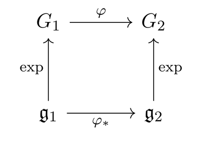
Actually, taking the tangent space at the identity is a functor. Consider a map $\varphi \colon G_1 \rightarrow G_2$ of Lie groups, with lie algebras $\mathfrak g_1$ and $\mathfrak g_2$. Because $\varphi$ is a group homomorphism, $G_1 \ni e_1 \mapsto e_2 \in G_2$. Now, by manifold theory we know that maps $f \colon M \rightarrow N$ between manifolds gives a linear map between the corresponding tangent spaces, say $Tf \colon T_pM \rightarrow T_{fp}N$. For us we obtain a linear map $$\varphi_\ast = T \varphi \colon \mathfrak g_1 \rightarrow \mathfrak g_2.$$ In fact, this $\varphi_\ast$ fits into a diagram

Here are a few more properties of $\exp$:

• $\exp(0) = e \in G$, which is immediate by looking at the constant trajectory $\phi_0(t) \equiv e$.
• $\exp'(x) = x \in \mathfrak g$, i.e. the total derivative $D\exp \colon \mathfrak g \rightarrow \mathfrak g$ is the identity. This is again by construction.
• In particular, by the inverse function theorem this implies that $\exp$ is a diffeomorphism in a neighborhood of $0 \in \mathfrak g$, onto a neighborhood of $e \in G$.
• $\exp$ commutes with the commutator. (By the above diagram.)

5. The commutator

Right now $\mathfrak g$ is still just a vector space, the tangent space. But now that there is map $\exp \colon \mathfrak g \rightarrow G$, we can use it to put a new operation on $\mathfrak g$, the so-called commutator.

The idea is follows: we want to “multiply” two elements of $\mathfrak g$. But $\mathfrak g$ is just a vector space, so we can’t do that. However, $G$ itself has a group multiplication, so we should pass to $G$ using $\exp$, use the multiplication in the group $G$ and then come back.

Here are the details. As we just mentioned, $\exp$ is a diffeomorphism near $e \in G$. So for $x$, $y$ close to the origin of $\mathfrak g$, we can look at $\exp(x)$ and $\exp(y)$, which are two elements of $G$ close to $e$. Multiplying them gives an element still close to $e$, so its equal to $\exp(z)$ for some unique $z$, call it $\mu(x,y)$.

One can show in fact that $\mu$ can be written as a Taylor series in two variables as $$\mu(x,y) = x + y + \frac{1}{2} [x,y] + \text{third order terms} + \dots$$ where $[x,y]$ is a skew-symmetric bilinear map, meaning $[x,y] = -[y,x]$. It will be more convenient to work with $[x,y]$ than $\mu(x,y)$ itself, so we give it a name:

Definition 17. This $[x,y]$ is called the commutator of $G$.

Now we know multiplication in $G$ is associative, so this should give us some nontrivial relation on the bracket $[,]$. Specifically, since $$\exp(x) \left( \exp(y) \exp(z) \right) = \left( \exp(x) \exp(y) \right) \exp(z).$$ we should have that $\mu(x, \mu(y,z)) = \mu(\mu(x,y), z)$, and this should tell us something. In fact, the claim is:

Theorem 18. The bracket $[,]$ satisfies the Jacobi identity $$[x,[y,z]] + [y,[z,x]] + [z,[x,y]] = 0.$$

Proof: Although I won’t prove it, the third-order terms (and all the rest) in our definition of $[x,y]$ can be written out explicitly as well: for example, for example, we actually have

$$\mu(x,y) = x + y + \frac{1}{2} [x,y] + \frac{1}{12} \left( [x, [x,y]] + [y,[y,x]] \right) + \text{fourth order terms} + \dots.$$

The general formula is called the Baker-Campbell-Hausdorff formula.

Then we can force ourselves to expand this using the first three terms of the BCS formula and then equate the degree three terms. The left-hand side expands initially as $\mu\left( x, y + z + \frac{1}{2} [y,z] + \frac{1}{12} \left( [y,[y,z]] + [z,[z,y] \right) \right)$, and the next step would be something ugly.

This computation is horrifying and painful, so I’ll pretend I did it and tell you the end result is as claimed. $\Box$

There is a more natural way to see why this identity is the “right one”; see Qiaochu. However, with this proof I want to make the point that this Jacobi identity is not our decision: instead, the Jacobi identity is forced upon us by associativity in $G$.

Example 19 (Examples of commutators attached to Lie groups)

• If $G$ is an abelian group, we have $-[y,x] = [x,y]$ by symmetry and $[x,y] = [y,x]$ from $\mu(x,y) = \mu(y,x)$. Thus $[x,y] = 0$ in $\mathfrak g$ for any abelian Lie group $G$.
• In particular, the brackets for $G \in \{\mathbb R, \mathbb C, S^1\}$ are trivial.
• Let $G = \operatorname{GL}(n, K)$. Then one can show that $$[T,S] = TS - ST \qquad \forall S, T \in \mathfrak{gl}(n, K).$$
• Ditto for $\operatorname{SL}(n, K)$.

In any case, with the Jacobi identity we can define an general Lie algebra as an intrinsic object with a Jacobi-satisfying bracket:

Definition 20. A Lie algebra over $k$ is a $k$-vector space equipped with a skew-symmetric bilinear bracket $[,]$ satisfying the Jacobi identity.

A morphism of Lie algebras and preserves the bracket.

Note that a Lie algebra may even be infinite-dimensional (even though we are assuming $G$ is finite-dimensional, so that they will never come up as a tangent space).

Example 21 (Associative algebra $\rightarrow$ Lie algebra)

Any associative algebra $A$ over $k$ can be made into a Lie algebra by taking the same underlying vector space, and using the bracket $[a,b] = ab - ba$.

6. The fundamental theorems

We finish this list of facts by stating the three “fundamental theorems” of Lie theory. They are based upon the functor $$\mathscr{L} \colon G \mapsto T_e G$$ we have described earlier, which is a functor

• from the category of Lie groups
• into the category of finite-dimensional Lie algebras.

The first theorem requires the following definition:

Definition 22. A Lie subgroup $H$ of a Lie group $G$ is a subgroup $H$ such that the inclusion map $H \hookrightarrow G$ is also an injective immersion.

A Lie subalgebra $\mathfrak h$ of a Lie algebra $\mathfrak g$ is a vector subspace preserved under the bracket (meaning that $[\mathfrak h, \mathfrak h] \subseteq \mathfrak h$).

Theorem 23 (Lie I)

Let $G$ be a real or complex Lie group with Lie algebra $\mathfrak g$. Then given a Lie subgroup $H \subseteq G$, the map $$H \mapsto \mathscr{L}(H) \subseteq \mathfrak g$$ is a bijection between Lie subgroups of $G$ and Lie subalgebras of $\mathfrak g$.

Theorem 24 (The Lie functor is an equivalence of categories)

Restrict $\mathscr{L}$ to a functor

• from the category of simply connected Lie groups over $K$
• to the category of finite-dimensional Lie algebras over $K$.

Then

1. (Lie II) $\mathscr{L}$ is fully faithful, and
2. (Lie III) $\mathscr{L}$ is essentially surjective on objects.

If we drop the “simply connected” condition, we obtain a functor which is faithful and exact, but not full: non-isomorphic Lie groups can have isomorphic Lie algebras (one example is $\operatorname{SO}(3)$ and $\operatorname{SU}(2)$).