More than six months late, but here are notes from the combinatorial nullsetllensatz talk I gave at the student colloquium at MIT. This was also my term paper for 18.434, “Seminar in Theoretical Computer Science”.

1. Introducing the choice number

One of the most fundamental problems in graph theory is that of a graph coloring, in which one assigns a color to every vertex of a graph so that no two adjacent vertices have the same color. The most basic invariant related to the graph coloring is the chromatic number:

Definition 1. A simple graph $G$ is $k$-colorable if it’s possible to properly color its vertices with $k$ colors. The smallest such $k$ is the chromatic number $\chi(G)$.

In this exposition we study a more general notion in which the set of permitted colors is different for each vertex, as long as at least $k$ colors are listed at each vertex. This leads to the notion of a so-called choice number, which was introduced by Erdös, Rubin, and Taylor.

Definition 2. A simple graph $G$ is $k$-choosable if its possible to properly color its vertices given a list of $k$ colors at each vertex. The smallest such $k$ is the choice number $\operatorname{ch}(G)$.

Example 3. We have $\operatorname{ch}(C_{2n}) = \chi(C_{2n}) = 2$ for any integer $n$ (here $C_{2n}$ is the cycle graph on $2n$ vertices). To see this, we only have to show that given a list of two colors at each vertex of $C_{2n}$, we can select one of them.

• If the list of colors is the same at each vertex, then since $C_{2n}$ is bipartite, we are done.
• Otherwise, suppose adjacent vertices $v_1$, $v_{2n}$ are such that some color at $c$ is not in the list at $v_{2n}$. Select $c$ at $v_1$, and then greedily color in $v_2$, …, $v_{2n}$ in that order.

We are thus naturally interested in how the choice number and the chromatic number are related. Of course we always have $$\operatorname{ch}(G) \ge \chi(G).$$ Näively one might expect that we in fact have an equality, since allowing the colors at vertices to be different seems like it should make the graph easier to color. However, the following example shows that this is not the case.

Example 4 (Erdös)

Let $n \ge 1$ be an integer and define $$G = K_{n^n, n}.$$ We claim that for any integer $n \ge 1$ we have $$\operatorname{ch}(G) \ge n+1 \quad\text{and}\quad \chi(G) = 2.$$ The latter equality follows from $G$ being partite.

Now to see the first inequality, let $G$ have vertex set $U \cup V$, where $U$ is the set of functions $u : [n] \rightarrow [n]$ and $V = [n]$. Then consider $n^2$ colors $C_{i,j}$ for $1 \le i, j \le n$. On a vertex $u \in U$, we list colors $C_{1,u(1)}$, $C_{2,u(2)}$, …, $C_{n,u(n)}$. On a vertex $v \in V$, we list colors $C_{v,1}$, $C_{v,2}$, …, $C_{v,n}$. By construction it is impossible to properly color $G$ with these colors.

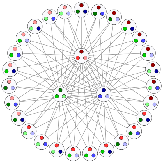
The case $n = 3$ is illustrated in the figure below (image in public domain).

This surprising behavior is the subject of much research: how can we bound the choice number of a graph as a function of its chromatic number and other properties of the graph? We see that the above example requires exponentially many vertices in $n$.

Theorem 5 (Noel, West, Wu, Zhu)

If $G$ is a graph with $n$ vertices then

$$\chi(G) \le \operatorname{ch}(G) \le \max\left( \chi(G), \left\lceil \frac{\chi(G)+n-1}{3} \right\rceil \right).$$

In particular, if $n \le 2\chi(G)+1$ then $\operatorname{ch}(G) = \chi(G)$.

One of the most major open problems in this direction is the following.

Definition 6. A claw-free graph is a graph with no induced $K_{3,1}$. For example, the line graph (also called edge graph) of any simple graph $G$ is claw-free.

If $G$ is a claw-free graph, then it’s conjectured $\operatorname{ch}(G) = \chi(G)$. In particular, this conjecture implies that for edge coloring, the notions of “chromatic number” and “choice number” coincide.

In this exposition, we prove the following result of Alon.

Theorem 7 (Alon)

A bipartite graph $G$ is $\left\lfloor L(G) \right\rfloor+1$ choosable, where $$L(G) \overset{\mathrm{def}}{=} \max_{H \subseteq G} |E(H)|/|V(H)|$$ is half the maximum of the average degree of subgraphs $H$.

In particular, recall that a planar bipartite graph $H$ with $r$ vertices contains at most $2r-4$ edges. Thus for such graphs we have $L(G) \le 2$ and deduce:

Corollary 8. A planar bipartite graph is $3$-choosable.

This corollary is sharp, as it applies to $K_{2,4}$ which we have seen in Example 4 has $\operatorname{ch}(K_{2,4}) = 3$.

The rest of the paper is divided as follows. First, we begin in §2 by stating Theorem 9, the famous combinatorial nullstellensatz of Alon. Then in §3 and §4, we provide descriptions of the so-called graph polynomial, to which we then apply combinatorial nullstellensatz to deduce Theorem 18. Finally in §5, we show how to use Theorem 18 to prove Theorem 7.

2. Combinatorial Nullstellensatz

The main tool we use is the Combinatorial Nullestellensatz of Alon.

Theorem 9 (Combinatorial Nullstellensatz)

Let $F$ be a field, and let $f \in F[x_1, \dots, x_n]$ be a polynomial of degree $t_1 + \dots + t_n$. Let $S_1, S_2, \dots, S_n \subseteq F$ such that $\left\lvert S_i \right\rvert > t_i$ for all $i$.

Assume the coefficient of $x_1^{t_1}x_2^{t_2}\dots x_n^{t_n}$ of $f$ is not zero. Then we can pick $s_1 \in S_1$, …, $s_n \in S_n$ such that $$f(s_1, s_2, \dots, s_n) \neq 0.$$

Example 10. Let us give a second proof that $$\operatorname{ch}(C_{2n}) = 2$$ for every positive integer $n$. Our proof will be an application of the Nullstellensatz.

Regard the colors as real numbers, and let $S_i$ be the set of colors at vertex $i$ (hence $1 \le i \le 2n$, and $|S_i| = 2$). Consider the polynomial

$$f = \left( x_1-x_2 \right)\left( x_2-x_3 \right) \dots \left( x_{2n-1}-x_{2n} \right)\left( x_{2n}-x_1 \right)$$

The coefficient of $x_1^1 x_2^1 \dots x_{2n}^1$ is $2 \neq 0$. Therefore, one can select a color from each $S_i$ so that $f$ does not vanish.

3. The Graph Polynomial, and Directed Orientations

Motivated by Example 10, we wish to apply a similar technique to general graphs $G$. So in what follows, let $G$ be a (simple) graph with vertex set $\{1, \dots, n\}$.

Definition 11. The graph polynomial of $G$ is defined by $$f_G(x_1, \dots, x_n) = \prod_{\substack{(i,j) \in E(G) \\ i < j}} (x_i-x_j).$$

We observe that coefficients of $f_G$ correspond to differences in directed orientations. To be precise, we introduce the notation:

Definition 12. Consider orientations on the graph $G$ with vertex set $\{1, \dots, n\}$, meaning we assign a direction $v \rightarrow w$ to every edge of $G$ to make it into a directed graph $G$. An oriented edge is called ascending if $v \rightarrow w$ and $v \le w$, i.e. the edge points from the smaller number to the larger one.

Then we say that an orientation is

• even if there are an even number of ascending edges, and
• odd if there are an odd number of ascending edges.

Finally, we define

• $\mathop{\mathrm{DE}}_G(d_1, \dots, d_n)$ to the be set of all even orientations of $G$ in which vertex $i$ has indegree $d_i$.
• $\mathop{\mathrm{DO}}_G(d_1, \dots, d_n)$ to the be set of all odd orientations of $G$ in which vertex $i$ has indegree $d_i$.

Set $\mathop{\mathrm{D}}_G(d_1,\dots,d_n) = \mathop{\mathrm{DE}}_G(d_1,\dots,d_n) \cup \mathop{\mathrm{DO}}_G(d_1,\dots,d_n)$.

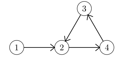
Example 13. Consider the following orientation:

There are exactly two ascending edges, namely $1 \rightarrow 2$ and $2 \rightarrow 4$. The indegrees of are $d_1 = 0$, $d_2 = 2$ and $d_3 = d_4 = 1$. Therefore, this particular orientation is an element of $\mathop{\mathrm{DE}}_G(0,2,1,1)$. In terms of $f_G$, this corresponds to the choice of terms

$$\left( x_1- \boldsymbol{x_2} \right) \left( \boldsymbol{x_2}-x_3 \right) \left( x_2-\boldsymbol{x_4} \right) \left( \boldsymbol{x_3}-x_4 \right)$$

which is a $+ x_2^2 x_3 x_4$ term.

Lemma 14. In the graph polynomial of $G$, the coefficient of $x_1^{d_1} \dots x_n^{d_n}$ is

$$\left\lvert \mathop{\mathrm{DE}}_G(d_1, \dots, d_n) \right\rvert - \left\lvert \mathop{\mathrm{DO}}_G(d_1, \dots, d_n) \right\rvert.$$

Proof: Consider expanding $f_G$. Then each expanded term corresponds to a choice of $x_i$ or $x_j$ from each $(i,j)$, as in Example 13. The term has coefficient $+1$ is the orientation is even, and $-1$ if the orientation is odd, as desired. $\Box$

Thus we have an explicit combinatorial description of the coefficients in the graph polynomial $f_G$.

4. Coefficients via Eulerian Suborientations

We now give a second description of the coefficients of $f_G$.

Definition 15. Let $D \in \mathop{\mathrm{D}}_G(d_1, \dots, d_n)$, viewed as a directed graph. An Eulerian suborientation of $D$ is a subgraph of $D$ (not necessarily induced) in which every vertex has equal indegree and outdegree. We say that such a suborientation is

• even if it has an even number of edges, and
• odd if it has an odd number of edges.

Note that the empty suborientation is allowed. We denote the even and odd Eulerian suborientations of $D$ by $\mathop{\mathrm{EE}}(D)$ and $\mathop{\mathrm{EO}}(D)$, respectively.

Eulerian suborientations are brought into the picture by the following lemma.

Lemma 16. Assume $D \in \mathop{\mathrm{DE}}_G(d_1, \dots, d_n)$. Then there are natural bijections

$$\begin{aligned} \mathop{\mathrm{DE}}_G(d_1, \dots, d_n) &\rightarrow \mathop{\mathrm{EE}}(D) \\ \mathop{\mathrm{DO}}_G(d_1, \dots, d_n) &\rightarrow \mathop{\mathrm{EO}}(D). \end{aligned}$$

Similarly, if $D \in \mathop{\mathrm{DO}}_G(d_1, \dots, d_n)$ then there are bijections

$$\begin{aligned} \mathop{\mathrm{DE}}_G(d_1, \dots, d_n) &\rightarrow \mathop{\mathrm{EO}}(D) \\ \mathop{\mathrm{DO}}_G(d_1, \dots, d_n) &\rightarrow \mathop{\mathrm{EE}}(D). \end{aligned}$$

Proof: Consider any orientation $D' \in \mathop{\mathrm{D}}_G(d_1, \dots, d_n)$. Then we define a suborietation of $D$, denoted $D \rtimes D'$, by including exactly the edges of $D$ whose orientation in $D'$ is in the opposite direction. It’s easy to see that this induces a bijection

$$D \rtimes - : \mathop{\mathrm{D}}_G(d_1, \dots, d_n) \rightarrow \mathop{\mathrm{EE}}(D) \cup \mathop{\mathrm{EO}}(D)$$

Moreover, remark that

• $D \rtimes D'$ is even if $D$ and $D'$ are either both even or both odd, and
• $D \rtimes D'$ is odd otherwise.

The lemma follows from this. $\Box$

Corollary 17. In the graph polynomial of $G$, the coefficient of $x_1^{d_1} \dots x_n^{d_n}$ is

$$\pm \left( \left\lvert \mathop{\mathrm{EE}}(D) \right\rvert - \left\lvert \mathop{\mathrm{EO}}(D) \right\rvert \right)$$

where $D \in \mathop{\mathrm{D}}_G(d_1, \dots, d_n)$ is arbitrary.

Proof: Combine Lemma 14 and Lemma 16. $\Box$

We now arrive at the main result:

Theorem 18. Let $G$ be a graph on $\{1, \dots, n\}$, and let $D \in \mathop{\mathrm{D}}_G(d_1, \dots, d_n)$ be an orientation of $G$. If $\left\lvert \mathop{\mathrm{EE}}(D) \right\rvert \neq \left\lvert \mathop{\mathrm{EO}}(D) \right\rvert$, then given a list of $d_i+1$ colors at each vertex of $G$, there exists a proper coloring of the vertices of $G$.

In particular, $G$ is $(1+\max_i d_i)$-choosable.

Proof: Combine Corollary 17 with Theorem 9. $\Box$

5. Finding an orientation

Armed with Theorem 18, we are almost ready to prove Theorem 7. The last ingredient is that we need to find an orientation on $G$ in which the maximal degree is not too large. This is accomplished by the following.

Lemma 19. Let $L(G) \overset{\mathrm{def}}{=} \max_{H \subseteq G} |E(H)|/|V(H)|$ as in Theorem 7. Then $G$ has an orientation in which every indegree is at most $\left\lceil L(G) \right\rceil$.

Proof: This is an application of Hall’s marriage theorem.

Let $d = \left\lceil L(G) \right\rceil \ge L(G)$. Construct a bipartite graph

$$E \cup X \qquad \text{where}\qquad E = E(G) \quad\text{ and }\quad X = \underbrace{V(G) \sqcup \dots \sqcup V(G)}_{d \text{ times}}.$$

Connect $e \in E$ and $v \in X$ if $v$ is an endpoint of $e$. Since $d \ge L(G)$ we satisfy Hall’s condition (as $L(G)$ is a condition for all subgraphs $H \subseteq G$) and can match each edge in $E$ to a (copy of some) vertex in $X$. Since there are exactly $d$ copies of each vertex in $X$, the conclusion follows. $\Box$

Now we can prove Theorem 7.

Proof: According to Lemma 19, pick $D \in \mathop{\mathrm{D}}_G(d_1, \dots, d_n)$ where $\max d_i \le \left\lceil L(G) \right\rceil$. Since $G$ is bipartite, we obviously have $\mathop{\mathrm{EO}}(D) = \varnothing$, since $G$ cannot have any odd cycles. So Theorem 18 applies and we are done. $\Box$