Here I talk about my first project at the Emory REU. Prerequisites for this post: some familiarity with number fields.

1. Motivation: Arithmetic Progressions

Given a property $P$ about primes, there’s two questions we can ask:

1. How many primes $\le x$ are there with this property?
2. What’s the least prime with this property?

As an example, consider an arithmetic progression $a$, $a+d$, …, with $a < d$ and $\gcd(a,d) = 1$. The strong form of Dirichlet’s Theorem tells us that basically, the number of primes $\equiv a \pmod d$ is $\frac 1d$ the total number of primes. Moreover, the celebrated Linnik’s Theorem tells us that the first prime is $O(d^L)$ for a fixed $L$, with record $L = 5$.

As I talked about last time on my blog, the key ingredients were:

• Introducing Dirichlet characters $\chi$, which are periodic functions modulo $q$. One uses this to get the mod $q$ into the problem.
• Introducing an $L$-function $L(s, \chi)$ attached to $\chi$.
• Using complex analysis (Cauchy’s Residue Theorem) to boil the proof down to properties of the zeros of $L(s, \chi)$.

With that said, we now move to the object of interest: elliptic curves.

2. Counting Primes

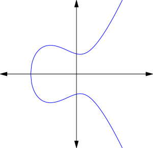
Let $E$ be an elliptic curve over $\mathbb Q$, which for our purposes we can think of concretely as a curve in Weirestrass form $$y^2 = x^3 + Ax + B$$ where the right-hand side has three distinct complex roots (viewed as a polynomial in $x$). If we are unlucky enough that the right-hand side has a double root, then the curve ceases to bear the name “elliptic curve” and instead becomes singular.

Here’s a natural number theoretic question: for any rational prime $p$, how many solutions does $E$ have modulo $p$?

To answer this it’s helpful to be able to think over an arbitrary field $F$. While we’ve written our elliptic curve $E$ as a curve over $\mathbb Q$, we could just as well regard it as a curve over $\mathbb C$, or as a curve over $\mathbb Q(\sqrt 2)$. Even better, since we’re interested in counting solutions modulo $p$, we can regard this as a curve over $\mathbb F_p$. To make this clear, we will use the notation $E/F$ to signal that we are thinking of our elliptic curve over the field $F$. Also, we write $\#E(F)$ to denote the number of points of the elliptic curve over $F$ (usually when $F$ is a finite field). Thus, the question boils down to computing $\#E(\mathbb F_p)$.

Anyways, the question above is given by the famous Hasse bound, and in fact it works over any number field!

Theorem 1 (Hasse Bound)

Let $K$ be a number field, and let $E/K$ be an elliptic curve. Consider any prime ideal $\mathfrak p \subseteq \mathcal O_K$ which is not ramified. Then we have $$\#E(\mathbb F_\mathfrak p) = \mathrm{N}\mathfrak p + 1 - a_\mathfrak p$$ where $\left\lvert a_\mathfrak p \right\rvert \le 2\sqrt{\mathrm{N}\mathfrak p}$.

Here $\mathbb F_\mathfrak p = \mathcal O_K / \mathfrak p$ is the field of $\mathrm{N}\mathfrak p$ elements. The extra “$+1$” comes from a point at infinity when you complete the elliptic curve in the projective plane.

Here, the ramification means what you might guess. Associated to every elliptic curve over $\mathbb Q$ is a conductor $N$, and a prime $p$ is ramified if it divides $N$. The finitely many ramified primes are the “bad” primes for which something breaks down when we take modulo $p$ (for example, perhaps the curve becomes singular).

In other words, for the $\mathbb Q$ case, except for finitely many bad primes $p$, the number of solutions is $p + 1 + O(\sqrt p)$, and we even know the implied $O$-constant to be $2$.

Now, how do we predict the error term?

3. The Sato-Tate Conjecture

For elliptic curves over $\mathbb Q$, we the Sato-Tate conjecture (which recently got upgraded to a theorem) more or less answers the question. But to state it, I have to introduce a new term: an elliptic curve $E/\mathbb Q$, when regarded over $\mathbb C$, can have complex multiplication (abbreviated CM). I’ll define this in just a moment, but for now, the two things to know are

• CM curves are “special cases”, in the sense that a randomly selected elliptic curve won’t have CM.
• It’s not easy in general to tell whether a given elliptic curve has CM.

Now I can state the Sato-Tate result. It is most elegantly stated in terms of the following notation: if we define $a_p = p + 1 - \#E(\mathbb F_p)$ as above, then there is a unique $\theta_p \in [0,\pi]$ which obeys $$a_p = 2 \sqrt p \cos \theta_p.$$

Theorem 2 (Sato-Tate)

Fix an elliptic curve $E/\mathbb Q$ which does not have CM (when regarded over $\mathbb C$). Then as $p$ varies across unramified primes, the asymptotic probability that $\theta_p \in [\alpha, \beta]$ is $$\frac{2}{\pi} \int_{[\alpha, \beta]} \sin^2\theta_p.$$ In other words, $\theta_p$ is distributed according to the measure $\sin^2\theta$.

Now, what about the CM case?

4. CM Elliptic Curves

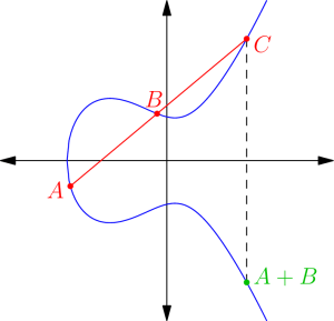
Consider an elliptic curve $E/\mathbb Q$ but regard it as a curve over $\mathbb C$. It’s well known that elliptic curves happen to have a group law: given two points on an elliptic curve, you can add them to get a third point. (If you’re not familiar with this, Wikipedia has a nice explanation). So elliptic curves have more structure than just their set of points: they form an abelian group; when written in Weirerstrass form, the identity is the point at infinity.

Letting $A = (A, +)$ be the associated abelian group, we can look at the endomorphisms of $E$ (that is, homomorphisms $A \rightarrow A$). These form a ring, which we denote $\operatorname{End}(E)$. An example of such an endomorphism is $a \mapsto n \cdot a$ for an integer $n$ (meaning $a+\dots+a$, $n$ times). In this way, we see that $\mathbb Z \subseteq \operatorname{End}(E)$.

Most of the time we in fact have $\operatorname{End}(E) \cong \mathbb Z$. But on occasion, we will find that $\operatorname{End}(E)$ is congruent to $\mathcal O_K$, the ring of integers of a number field $K$. This is called complex multiplication by $K$.

Intuitively, this CM is special (despite being rare), because it means that the group structure associated to $E$ has a richer set of symmetry. For CM curves over any number field, for example, the Sato-Tate result becomes very clean, and is considerably more straightforward to prove.

Here’s an example. The elliptic curve $$E : y^2 = x^3 - 17 x$$ of conductor $N = 2^6 \cdot 17^2$ turns out to have $$\operatorname{End}(E) \cong \mathbb Z[i]$$ i.e. it has complex multiplication has $\mathbb Z[i]$. Throwing out the bad primes $2$ and $17$, we compute the first several values of $a_p$, and something bizarre happens. For the $3$ mod $4$ primes we get

$$\begin{aligned} a_{3} &= 0 & a_{7} &= 0 & a_{11} &= 0 \\ a_{19} &= 0 & a_{23} &= 0 & a_{31} &= 0 \end{aligned}$$

and for the $1$ mod $4$ primes we have

$$\begin{aligned} a_5 &= 4 \\ a_{13} &= 6 \\ a_{29} &= 4 \\ a_{37} &= 12 \\ a_{41} &= -8 \end{aligned}$$

Astonishingly, the vanishing of $a_p$ is controlled by the splitting of $p$ in $\mathbb Z[i]$! In fact, this holds more generally. It’s a theorem that for elliptic curves $E/\mathbb Q$ with CM, we have $\operatorname{End}(E) \cong \mathcal O_K$ where $K$ is some quadratic imaginary number field which is also a PID, like $\mathbb Z[i]$. Then $\mathcal O_K$ governs how the $a_p$ behave:

Theorem 3 (Sato-Tate Over CM)

Let $E/\mathbb Q$ be a fixed elliptic curve with CM by $\mathcal O_K$. Let $\mathfrak p$ be a unramified prime of $\mathcal O_K$.

1. If $\mathfrak p$ is inert, then $a_\mathfrak p = 0$ (i.e. $\theta_\mathfrak p = \frac{1}{2}\pi$).
2. If $\mathfrak p$ is split, then $\theta_\mathfrak p$ is uniform across $[0, \pi]$.

I’m told this is much easier to prove than the usual Sato-Tate.

But there’s even more going on in the background. If I look again at $a_p$ where $p \equiv 1 \pmod 4$, I might recall that $p$ can be written as the sum of squares, and construct the following table:

$$\begin{array}{rrl} p & a_p & x^2+y^2 \\ 5 & 4 & 2^2 + 1^2 \\ 13 & 6 & 3^2 + 2^2 \\ 29 & 4 & 2^2 + 5^2 \\ 37 & 12 & 6^2 + 1^2 \\ 41 & -8 & 4^2 + 5^2 \\ 53 & 14 & 7^2 + 2^2 \\ 61 & 12 & 6^2 + 5^2 \\ 73 & -16 & 8^2 + 3^2 \\ 89 & -10 & 5^2 + 8^2 \\ \end{array}$$

Each $a_p$ is double one of the terms! There is no mistake: the $a_p$ are also tied to the decomposition of $p = x^2+y^2$. And this works for any number field.

What’s happening? The main idea is that looking at a prime ideal $\mathfrak p = (x+yi)$, $a_\mathfrak p$ is related to the argument of the complex number $x+yi$ in some way. Of course, there are lots of questions unanswered (how to pick the $\pm$ sign, and which of $x$ and $y$ to choose) but there’s a nice way to package all this information, as I’ll explain momentarily.

(Aside: I think the choice of having $x$ be the odd or even number depends precisely on whether $p$ is a quadratic residue modulo $17$, but I’ll have to check on that.)

5. $L$-Functions

I’ll just briefly explain where all this is coming from, and omit lots of details (in part because I don’t know all of them). Let $E/\mathbb Q$ be an elliptic curve with CM by $\mathcal O_K$. We can define an associated $L$-function

$$L(s, E/K) = \prod_\mathfrak p \left( 1 - \frac{a_\mathfrak p}{(\mathrm{N}\mathfrak p)^{s+\frac{1}{2}}} + \frac{1}{(\mathrm{N}\mathfrak p)^{2s}} \right)$$

(actually this isn’t quite true actually, some terms change for ramified primes $\mathfrak p$).

At the same time there’s a notion of a Hecke Grössencharakter $\xi$ on a number field $K$ – a higher dimensional analog of the Dirichlet characters we used on $\mathbb Z$ to filter modulo $q$. For our purposes, think of it as a multiplicative function which takes in ideals of $\mathcal O_K$ and returns complex numbers of norm $1$. Like Dirichlet characters, each $\xi$ gets a Hecke $L$-function $$L(s, \xi) = \prod_\mathfrak p \left( 1 - \frac{\xi(\mathfrak p)}{(\mathrm{N}\mathfrak p)^s} \right)$$ which again extends to a meromorphic function on the entire complex plane.

Now the great theorem is:

Theorem 4 (Deuring)

Let $E/\mathbb Q$ have CM by $\mathcal O_K$. Then $$L(s,E/K) = L(s, \xi)L(s, \overline{\xi})$$ for some Hecke Grössencharakter $\xi$.

Using the definitions given above and equating the Euler products at an unramified $\mathfrak p$ gives

$$1 - \frac{a_\mathfrak p}{(\mathrm{N}\mathfrak p)^{s+\frac{1}{2}}} + \frac{1}{(\mathrm{N}\mathfrak p)^{2s}} = \left( 1 - \frac{\xi(\mathfrak p)}{(\mathrm{N}\mathfrak p)^s} \right) \left( 1 - \frac{\overline{\xi(\mathfrak p)}}{(\mathrm{N}\mathfrak p)^s} \right)$$

Upon recalling that $a_\mathfrak p = 2 \sqrt{\mathrm{N}\mathfrak p} \cos \theta_\mathfrak p$, we derive $$\xi(\mathfrak p) = \exp(\pm i \theta_\mathfrak p).$$ This is enough to determine the entire $\xi$ since $\xi$ is multiplicative.

So this is the result: let $E/\mathbb Q$ be an elliptic curve of conductor $N$. Given our quadratic number field $K$, we define a map $\xi$ from prime ideals of $\mathcal O_K$ to the unit circle in $\mathbb C$ by

$$\mathfrak p \mapsto \begin{cases} \exp(\pm i \theta_\mathfrak p) & \gcd(\mathrm{N}\mathfrak p, N) = 1 \\ 0 & \gcd(\mathrm{N}\mathfrak p, N) > 1. \end{cases}$$

Thus $\xi$ is a Hecke Grössencharakter for some choice of $\pm$ at each $\mathfrak p$.

It turns out furthermore that $\xi$ has frequency $1$, which roughly means that the argument of $\xi\left( (\pi) \right)$ is related to $1$ times the argument of $\pi$ itself. This fact is what explains the mysterious connection between the $a_p$ and the solutions above.

6. Linnik-Type Result

With this in mind, I can now frame the main question: suppose we have an interval $[\alpha, \beta] \subset [0,\pi]$. What’s the first prime $p$ such that $\theta_p \in [\alpha, \beta]$? We’d love to have some analog of Linnik’s Theorem here.

This was our project and the REU, and Ashvin, Peter and I proved that

Theorem 5. If a rational $E$ has CM then the least prime $p$ with $\theta_p \in [\alpha,\beta]$ is $$\ll \left( \frac{N}{\beta-\alpha} \right)^A.$$

I might blog later about what else goes into the proof of this… but Deuring’s result is one key ingredient, and a proof of an analogous theorem for non-CM curves would have to be very different.